Point Operation
Point Operation
Point operation is a simple operation that is applied to each pixel in an image. Let \(r\) be the pixel value of the input image and \(s\) be the pixel value of the output image. The point operation can be expressed as \(s = T(r)\), where \(T\) is the transformation function. The transformation function can be a linear or nonlinear function, depending on the application.
Linear Transformation
\[s = T(r) = ar + b\]Segmental Linear Transformation
\[s = T(r) = \begin{cases} a_1 r + b_1, & \text{if } r < r_1 \\ a_2 r + b_2, & \text{if } r_1 \leq r < r_2 \\ a_3 r + b_3, & \text{if } r_2 \leq r < r_3 \\ \vdots \\ a_n r + b_n, & \text{if } r_{n-1} \leq r < r_n \\ a_{n+1} r + b_{n+1}, & \text{if } r \geq r_n \end{cases}\]Nonlinear Transformation
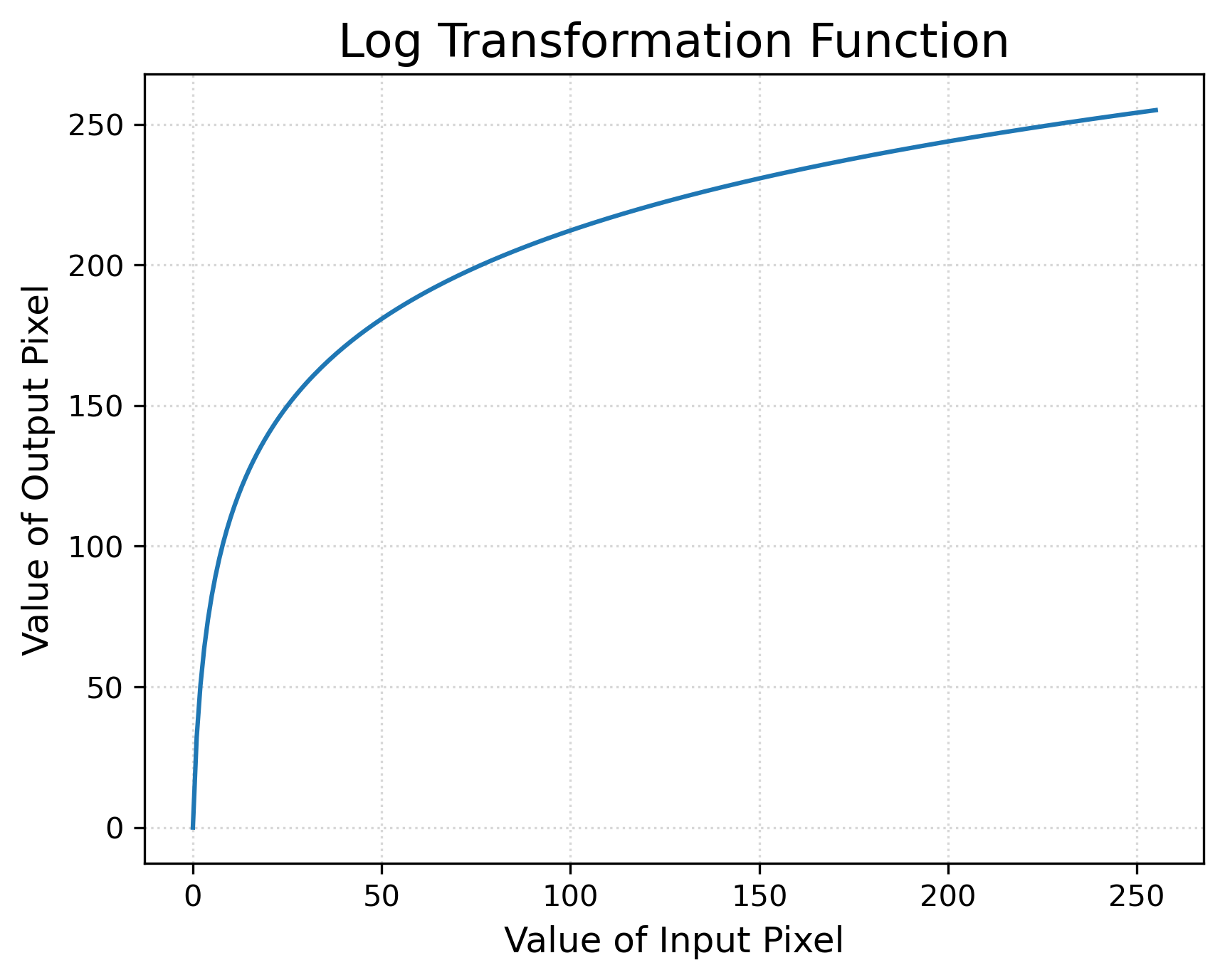
Log Transformation
\[s = T(r) = c \log(1 + r)\]
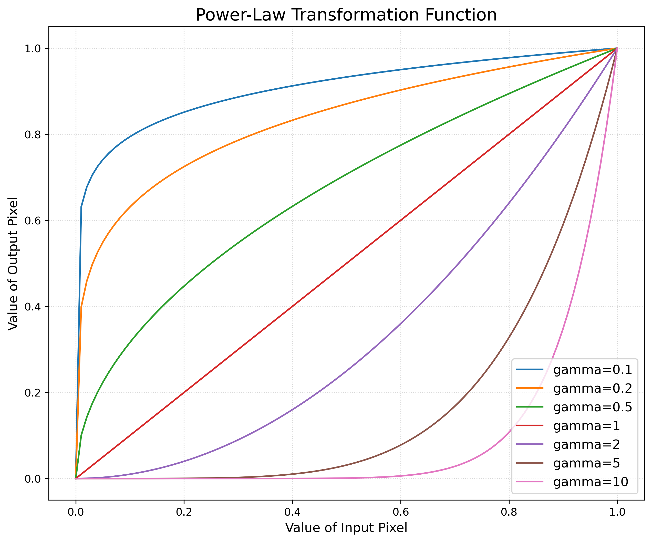
Power-Law (Gamma) Transformation
\[s = T(r) = cr^{\gamma}\]
Grayscale Threshold Transformation
\[s = T(r) = \begin{cases} 0, & \text{if } r < T \\ 255, & \text{if } r \geq T \end{cases}\]Histogram Equalization
Let \(r\) be a continuous variable limited to the range \([0, L-1]\), where \(L\) is the number of gray levels. The probability density function (PDF) of \(r\) is \(p_r(r)\), and the cumulative distribution function (CDF) of \(r\) is \(P_r(r)\). The PDF and CDF are defined as follows:
\[\begin{aligned} P_r(r) &= \int_{-\infty}^{r} p_r(w) dw\\ &= \int_{0}^{r} p_r(w) dw\\ \end{aligned}\]Now let \(s=(L-1)P_r(r)\) is a transformation function, \(s\) is limited to the range \([0, L-1]\), and the PDF of \(s\) is \(p_s(s)\). We can derive the PDF of \(s\) as follows:
\[p_s(s) = \frac{dP_s(s)}{ds} = \frac{dP_r(r)}{dr} \frac{dr}{ds} = p_r(r) \frac{dr}{ds}\]Then PDF of \(s\) can be expressed as follows:
\[\begin{aligned} \frac{ds}{dr} &= \frac{d}{dr} (L-1)P_r(r)\\ &= (L-1) \frac{dP_r(r)}{dr}\\ &= (L-1) p_r(r)\\ p_s(s) &= p_r(r) \frac{dr}{ds}\\ &= p_r(r) \frac{1}{\frac{ds}{dr}}\\ &= p_r(r) \frac{1}{(L-1) p_r(r)}\\ &= \frac{1}{L-1} \end{aligned}\]So the PDF of \(s\) is a uniform distribution. If we extend the case to discrete variables:
\[\begin{aligned} p_r(r) &= \frac{n_r}{MN}\\ P_r(r) &= \sum_{j=0}^{r} p_r(j)\\ s &= (L-1)P_r(r)\\ &= (L-1) \sum_{j=0}^{r} p_r(j)\\ &= (L-1) \sum_{j=0}^{r} \frac{n_j}{MN}\\ &= \frac{L-1}{MN} \sum_{j=0}^{r} n_j\\ \end{aligned}\]Since \(s\) must be an integer, we can round \(s\) to the nearest integer:
\[s = \left\lfloor \frac{L-1}{MN} \sum_{j=0}^{r} n_j + \frac{1}{2} \right\rfloor\]Let \(L=8\), \(M=N=64\), we can get a 3-bit image distribution.
| \(r\) | \(n_r\) | \(p_r(r)\) | \(P_r(r)\) | \(T(r)\) | \(s\) |
|---|---|---|---|---|---|
| 0 | 500 | 0.1221 | 0.1221 | 0.8545 | 1 |
| 1 | 200 | 0.0488 | 0.1709 | 1.1963 | 1 |
| 2 | 256 | 0.0625 | 0.2334 | 1.6338 | 2 |
| 3 | 384 | 0.0938 | 0.3272 | 2.2904 | 2 |
| 4 | 512 | 0.1250 | 0.4522 | 3.1654 | 3 |
| 5 | 640 | 0.1563 | 0.6085 | 4.2595 | 4 |
| 6 | 768 | 0.1875 | 0.7960 | 5.5720 | 6 |
| 7 | 836 | 0.2041 | 1.0000 | 7.0000 | 7 |
Histogram Matching
Histogram matching is a method to match the histogram of an input image to the histogram of a reference image where histogram equalization is applied. Let \(r\) be the input and \(z\) be the output, the PDF of \(z\) is already known.
\[s = T(r) = (L-1)\int_{0}^{r} p_r(w) dw\]The CDF of \(z\) is expected to be the same as the CDF of \(r\):
\[G(z) = (L-1)\int_{0}^{z} p_z(w) dw = s\]Since we got the relation between \(z\) and \(s\). we can derive the transformation function \(z = G^{-1}(s)\).
\[z = G^{-1}(T(r)) = G^{-1}(s)\]If we extend the case to discrete variables, all we need to do is to find the histogram equalization transformation function of the input image and the reference image, and then find the mapping between the two transformation functions \(s\) and \(G(z)\), then we can get the transformation from \(r\) to \(z\). The goal of histogram matching is to transform \(r\) to \(z\) as close as possible.