Evaluation in Data Science
Classification
Cross Entropy
\[\text{Cross Entropy} = - \sum_{i=1}^{n} y_i \ln(p_i)\]For binary classification, the cross entropy is
\[\text{Cross Entropy} = - y \ln(p) - (1 - y) \ln(1 - p)\]For multi-class classification, the cross entropy is
\[\text{Cross Entropy} = - \sum_{i=1}^{n}\sum_{j=1}^{m} y_{ij} \ln(p_{ij})\]where \(n\) is the number of samples, \(m\) is the number of classes, \(y_{ij}\) is the ground truth label of the \(i\)-th sample for the \(j\)-th class, and \(p_{ij}\) is the predicted probability of the \(i\)-th sample for the \(j\)-th class.
Confusion Matrix
Confusion matrix is a table that is often used to describe the performance of a classification model on a set of test data for which the true values are known. It is a 2x2 matrix for binary classification, and a \(n \times n\) matrix for multi-class classification.
| Actual Positive | Actual Negative | |
|---|---|---|
| Predicted Positive | True Positive (TP) | False Positive (FP) |
| Predicted Negative | False Negative (FN) | True Negative (TN) |
- True Positive (TP): The number of correct predictions that an instance is positive.
- False Positive (FP): The number of incorrect predictions that an instance is positive.
- False Negative (FN): The number of incorrect predictions that an instance is negative.
- True Negative (TN): The number of correct predictions that an instance is negative.
Accuracy
\[\text{Accuracy} = \frac{TP + TN}{TP + TN + FP + FN}\]Precision
\[\text{Precision} = \frac{TP}{TP + FP}\]Recall
\[\text{Recall} = \frac{TP}{TP + FN}\]F1 Score
\[\text{F1 Score} = 2 \times \frac{\text{Precision} \times \text{Recall}}{\text{Precision} + \text{Recall}}\]More generally, \(F_\beta\) score is a weighted harmonic mean of precision and recall, where \(\beta\) is a parameter that adjusts the weight of recall in the combined score.
\[F_\beta = \frac{(1+\beta^2)*Precision*Recall}{\beta^2*Precision+Recall}\]MCC
\[\text{MCC} = \frac{TP \times TN - FP \times FN}{\sqrt{(TP + FP)(TP + FN)(TN + FP)(TN + FN)}}\]MAP
Average precision (AP) is the average of precision at each recall level. It is a single number used to summarize a precision-recall curve.
Let \(R\) be the set of actual positive samples, and \(P\) be the set of predicted positive samples. The precision of each sample in \(R\) is
\[\text{Precision}_i = \left \{ \begin{matrix} \frac{TP_i}{TP_i + FP_i} & \text{if } i \in P \\ 0 & \text{otherwise} \end{matrix} \right.\]where \(TP_i\) is the number of true positives in the top \(i\) predictions, and \(FP_i\) is the number of false positives in the top \(i\) predictions. AP is averaged over all actual positive samples, meaning that zeros are included in the average.
\[\text{AP} = \frac{1}{|R|} \sum_{r \in R} \text{Precision}(r)\]Mean average precision (MAP) is the mean of AP across multiple queries/labels, usually referred to as macro-averaging, the unweighted mean of AP across all queries/labels.
\[\text{MAP} = \frac{1}{|Q|} \sum_{q \in Q} \text{AP}(q)\]where \(Q\) is the set of queries/labels.
ROC-AUC
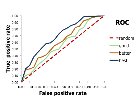
Receiver operating characteristic (ROC) curve is a curve that shows the performance of a binary classifier at different classification thresholds. Each point on the curve represents corresponding true positive rate (TPR, Recall, Sensitivity) and false positive rate (FPR) at a given threshold.
\[\text{TPR} = \frac{TP}{TP + FN}\] \[\text{FPR} = \frac{FP}{FP + TN}\]A simple way to plot ROC curve is to count the number of true positives \(P\) and true nagatives \(N\) of all samples. Then, set the interval of the x-axis to \(\frac{1}{N}\) and the interval of the y-axis to \(\frac{1}{P}\). Samples are sorted by their predicted probabilities in descending order. For each sample, if it is a true positive, move one step up; if it is a false positive, move one step right. The curve is the path of the points. And the path ends at (1, 1).
Area under the ROC curve (AUC) is the area under the ROC curve. It is a single number used to summarize a ROC curve. The larger the AUC, the better the performance of the classifier.

PR Curve
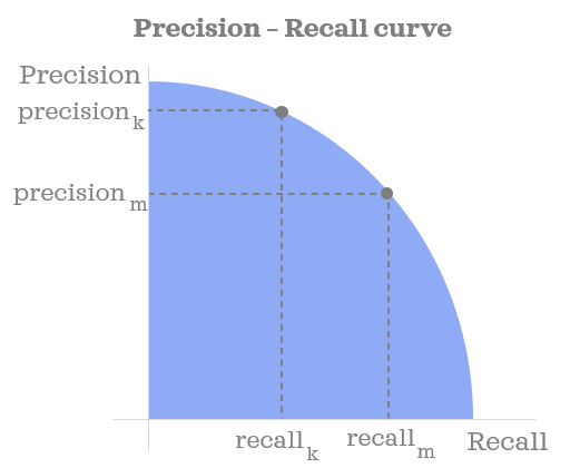
Precision-recall curve (PR curve) is a curve that shows the trade-off between precision and recall for different thresholds. Each point on the curve represents corresponding precision at a given recall level.
Break point is the point where the precision and recall are equal. The precision and recall at the break point are called break-even precision and break-even recall, respectively.

Multilabel Classification
Macro-averaging VS Micro-averaging
Macro-averaging is the unweighted mean of the per-class metric, while micro-averaging is the metric calculated globally by counting the specimens.
Regression
MSE
MAE
R2
MAPE
Clustering
Homework
ROC Curve
labels = [1, 0, 1, 0, 0, 0]
res_1 = [0.83, 0.78, 0.62, 0.48, 0.32, 0.22]
res_2 = [0.92, 0.62, 0.52, 0.49, 0.38, 0.28]
thresholds = [0, 0.2, 0.4, 0.6, 0.8, 1]
def get_points(labels, res, threshold):
    points = []
    for t in threshold:
        tp, fp, tn, fn = 0, 0, 0, 0
        for y, p in zip(labels, res):
            if p >= t:
                if y == 1:
                    tp += 1
                else:
                    fp += 1
            else:
                if y == 0:
                    tn += 1
                else:
                    fn += 1
        fpr = fp / (fp + tn)
        tpr = tp / (tp + fn)
        points.append((fpr, tpr))
    return points
points_1 = get_points(labels, res_1, thresholds)
points_2 = get_points(labels, res_2, thresholds)

plt.figure(figsize=(6, 4))
plt.plot([0, 1], [0, 1], 'k--')
plt.plot([p[0] for p in points_1], [p[1] for p in points_1], label='Model 1')
plt.plot([p[0] for p in points_2], [p[1] for p in points_2], label='Model 2')
plt.xlabel('False Positive Rate')
plt.ylabel('True Positive Rate')
plt.legend()
plt.show()
Overfitting and Underfitting
Overfitting occurs when a model learns the training data too well. This means that the model will perform well on the training data but poorly on the test data. Underfitting occurs when a model does not learn the training data well enough. This means that the model will perform poorly on both the training data and the test data.
Avoiding Overfitting
- Use a larger training set (reducing variance but not bias).
- Use a smaller model, i.e. fewer parameters.
- Use regularization.
- Use dropout.
- Use early stopping.
- Use feature selection or feature extraction.
- Use demensionality reduction.
Avoiding Underfitting
- Use a larger/more complex model, i.e. more parameters.
- Use more features.
- Use less regularization.
- Use more training epochs.
Bias and Variance
Bias is the difference between the expected prediction and the ground truth. Variance is the variability of the prediction.
Bias can be seen as the model’s ability to fit the training data, i.e. the training error. Variance can be seen as the model’s ability to generalize to new data, i.e. the difference between the training error and the test error.
Usually, a model with high bias has low variance, and a model with low bias has high variance. The goal is to find a model with low bias and low variance.
Variance-Bias Tradeoff
Let \(y\) be the ground truth, \(f(x)\) be the prediction, and \(y_D\) be the label of the training data. The expected prediction error can be decomposed as
\[\begin{aligned} \text{Bias} &= \mathbb{E}[f(x)] - y \\ \text{Variance} &= \mathbb{E}[(f(x) - \mathbb{E}[f(x)])^2] = \mathbb{E}[f(x)^2] - \mathbb{E}[f(x)]^2 \\ \epsilon &= y - y_D \sim \mathcal{N}(0, \sigma^2) \\ \mathbb{E}[(f(x) - y_D)^2] &= \mathbb{E}[(f(x) - \mathbb{E}[f(x)] + \mathbb{E}[f(x)] - y_D)^2] \\ &= \mathbb{E}[(f(x) - \mathbb{E}[f(x)])^2] + \mathbb{E}[(\mathbb{E}[f(x)] - y_D)^2] + 2\underbrace{\mathbb{E}[(f(x) - \mathbb{E}[f(x)])(\mathbb{E}[f(x)] - y_D)]}_{0} \\ &= \underbrace{\mathbb{E}[(f(x) - \mathbb{E}[f(x)])^2]}_{Var} + \mathbb{E}[(\mathbb{E}[f(x)] - y_D)^2] \\ &= \mathbb{E}[(f(x) - \mathbb{E}[f(x)])^2] + \mathbb{E}[(\mathbb{E}[f(x)] - y + y - y_D)^2] \\ &= \mathbb{E}[(f(x) - \mathbb{E}[f(x)])^2] + \mathbb{E}[(\mathbb{E}[f(x)] - y)^2] + \mathbb{E}[(y - y_D)^2] + 2\underbrace{\mathbb{E}[(\mathbb{E}[f(x)] - y)(y - y_D)]}_{0} \\ &= \underbrace{\mathbb{E}[(f(x) - \mathbb{E}[f(x)])^2]}_{Var} + \underbrace{\mathbb{E}[(\mathbb{E}[f(x)] - y)^2]}_{Bias^2} + \underbrace{\mathbb{E}[(y - y_D)^2]}_{\sigma^2} \\ \end{aligned}\]